ARR2019 – Areal Reduction Factors: interpolating between short and long duration ARFs

There are two equations provided for areal reduction factors (ARFs) in Australian Rainfall and Runoff 2019. One for long durations, greater than 1440 minutes (24 hours), and one for short durations, less than 720 minutes (12 hours).

To estimate ARFs between 12 hours and 24 hours we need to interpolate.  The recommendation in Australian Rainfall and Runoff 2019 is to do the required interpolation linearly (Podger et al., 2015)  Complicating matters, the short duration ARF equations are only suitable for catchment areas less than 1000 km² while long duration ARFs are available for catchments out to 30,000 km². The situation is summarised on Figure 1.

Surprisingly, ARR2019, recommends that interpolation can be used for catchment areas all the way out to 30,000 km².  That is, we can use the short duration equations as end points for interpolation for catchment areas larger than 1000 km².   This involves applying the short duration equations well beyond the range of the data that was used in their derivation (Stensmyr and Babister, 2015).

Figure 1: Application of short and long duration ARF equations as a function of catchment area and duration

Let’s start with the equations:

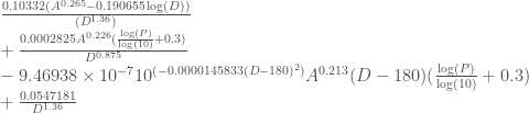
Short duration:

(equation 1)

Long duration:

(equation 2)

where, is area, is duration and is AEP.

The constants a, b, c, d, e, f, g, h, i depend on the region (Figure 2).  The values of these constants is shown below in a screen shot of Table 2.4.2 from ARR Book 2, Chapter 4.3.1.

Figure 2: ARF regions for Australia (Copy of ARR Book 2, Figure 2.4.1)

Here, we are interested in the case where area is larger than 1000 km² and duration falls between 12 and 24 hours.  Figure 2 shows an example for a catchment area of 30,000 km².  Between 12 and 24 hours, the ARFs are linearly interpolated between the long duration value at 24 hours and the short duration value calculated at 12 hours (solid line in Figure 2).  The short duration 12 hour value is subject to considerable uncertainty because the prediction equation was developed using data from catchments smaller than 1000 km² , much smaller than the 30,000 km² catchment area used here.

My first though was, if we require ARF estimates for durations between 12 and 24 hours, it would be better to just extend the long duration equations (the dashed line in Figure 2).   This would result in more conservative ARFs in the interpolation region.  And it is not obvious why extending the long duration equations is any worse than extrapolating short duration values and then interpolating from these values.  However, I now realise there are problems with this approach.

Figure 2: Interpolating between long and short duration ARFs

Extrapolating the long duration ARFs does not work for catchment areas close to 1000 km²  This can be seen on Figure 3.  For a catchment area of 1000 km² , both short and long duration ARFs can be calculated and the extrapolation between 12 and 24 hours is reasonable because the end points will be accurate.  Both equations are being used where there is data to support their derivation.   This is the red line on Figure 3.

Now consider the case for a catchment of 1100 km². The Short duration ARFs can no longer be calculated (because the limit of 1000 km²  is exceeded).   So, to calculate the ARF between 12 and 24 hours we could, either

1) Extend the long duration equation (dashed green line in Figure 3), or

2) Interpolate between the long duration value at 24 hours and the short duration value at 12 hours (the green solid line in Figure 3).

In this case, only approach 2 will work.  If we adopt approach 1, the ARFs for a larger 1100 km² catchment will exceed those for the smaller 1000 km² catchment (the dashed green line exceeds the solid red line).  This is not physically realistic.  As area increases, ARF is expected to decrease.

Figure 3: Interpolating ARF values between 12 and 24 hours for a 30,000 km² catchment

The upshot is, if you are working on catchments with areas only a bit larger than 1000 km² it would be best to do the ARF calculations using the recommended method, to avoid discontinuities in ARF values.

If you are working on catchments much larger than 1000 km² , and need to calculate an ARF between 12 and 24 hours, it may be worth checking the ARF values that result from extending the long-duration equations.   They will likely to be conservative, in that they will produce higher flood flows than the ARR recommended approach.  It is also in this region, i.e. where catchments area are much larger than 1000 km²,  that there is not strong justification for using the short duration equations as end points for the interpolation.  The support for these short duration equations reduces as catchment areas increase beyond the 1000 km²  limit that was used in their derivation.

Code to produce graphs is available as a Gist.

 

Reference

Stensmyr, P. and Babister, M. (2015) Short duration areal reduction factors.  Australian Rainfall and Runoff Revision Project 2: Spatial Patterns of Rainfall.  Stage 3 Report.  September 2015) (link).

Podger, S., Green, J., Stensmyr, P. and Babister, M. (2015).  Combining long and short duration areal reduction factors. Hydrology Water Resources Symposium (link to paper at Informit).

Comments on the report: “Impact of lower inflows on state shares under the Murray-Darling Basin Agreement”

First, this report is worth reading, its short and clearly written.  It’s produced by the Interim Inspector General of Murray-Darling Basin Water Resources, which is Mick Keelty AO, the former commissioner of the Australian Federal Police

The big story is that inflows to the Murray have decreased, a lot.

Inflows upstream of Albury

“…half of the driest years on record have occurred in the past 25 years”.

This sounds bad but its difficult to know what it means, however there is a telling graph of NSW inflows (Figure 1).  The last 20 years or so do not look some random perturbation of what has happened before.  This century looks very dry.  Counting the red bars suggests that 11 of the 12 driest years have occurred in the last 20 years.  And there is nothing in the historical record like the period from the mid 1990s to 2010/11 with year after year of low flows.

Figure 1: NSW inflows

Total inflows to the Murray

The report says: “More than half of the driest 10% of years in the historical record have occurred in the past two decades”.

So how unlikely is that?

Here is one interpretation.  The historical record is 126 years, from 1895 to 2020.  There would be, say, 13 years in “the driest 10% of years”, so “more than half” would be 7.

If we assume each year as independent, admittedly a strong assumption, then we can work out the probability of this occurring using the hypergeometric distribution*.

We need to calculate the probability of 7 or more “successes” from 13 items that could be labelled a success from a total population of 126.

The formula in excel is:  1-HYPGEOM.DIST(6,20,13,126, TRUE) = 0.000854

In R it’s 1-phyper(6, 13, 113, 20)

An alternative approach is to do a simulation.  Arrange the numbers 1 to 126 in random order and see how many of the numbers in the range 1 to 13 (representing the driest 10% of years) occur in the final 20 elements of that random series. Do this lots of times and count the number of occasions when this is 7 or more.

My answer is 0.000847 which is close to the theoretical answer so we are on the right track.

Here’s the code

Num_in_last_20 = function()  
{ 
  Ranks = sample(1:126, 126, replace = FALSE) 
  # sort the numbers 1 to 125 in random order 
  Last20 = Ranks[(length(Ranks) - 19): length(Ranks)] 
  # Get the last 20 elements 
  sum(Last20 %in% 1:13) # Number of ranks that are 13 or lower 
}  

# Repeat lots of times to determine the 
# probability there are 7 or more ranks less than 13 
  
mean(replicate(1000000, Num_in_last_20() >= 7))

These probabilities are likely underestimates, because the years are not independent, but they do suggest we should consider if there is a downward trend rather than just a random fluctuation.

Darling inflows

“Median inflows into the Menindee Lakes have reduced by about 80% in the last 20 years relative to the recorded period prior. Eight of the 13 driest years on record occurred in this period, most yielding zero or close to zero inflows.”

This is a similar situation to the total inflows to the Murray where 7 of the 13 driest years had occurred in the last 20 years.

So what is causing the low flows since 2000?  The report says there are numerous factors:

• low rainfall
• high temperatures
• catchment modification (including farm dams)
• increasing development
• floodplain harvesting
• changes in extraction rules in water sharing plans
• non-compliance.

Interestingly, there was virtually no change in inflows from the Snowy River.

Recommendation 1 of the report is:

“The MDBA should undertake further analysis of the causes of reduced inflows from the northern Basin and the extent to which this is affecting State water shares.”

It will be interesting to see what comes from that.

Pie chart and an alternative

There is lots of discussion on the internet about how pie charts are not a great way to show data.  People have difficulty judging angles and ordering pie slices from large to small (see the discussion in Wikipedia).  This report doesn’t shy away from a complicated pie chart.  The alternative column graph is shown below.  Do you think you could order the issues correctly just looking at the pie slices?

Code for this blog is available as a gist.

* Probability was calculated with some help from cross-validated.

ARR2019 – Areal Reduction Factors: wobbles in short duration ARFs

In the previous post we saw that short duration areal reduction factors (ARFs) looked a little wobbly for rare events (AEPs of 1% or less).  Here I look at this in more detail.

A plot of areal reduction factor against duration, for an AEP of 0.5% and for various areas, shows the issue (Figure 1). The long duration ARFs for durations greater than 1440 mins (24 hours), look to be well behaved.  But the short duration ARFs show a rapid and variable change in slope for durations between about 100 min and 720 min.  Also shown on Figure 1 is the gap between the short and long duration ARFs, between 720 min and 1440 min.  ARFs in this range are linearly interpolated. They don’t look linear on Figure 1 but that is because of the log scale on the x-axis.  I’ll write more about the interpolation between short and long duration ARFs in a later post.  Here we focus on the wobbles in the short duration ARFs.

Figure 1: Areal reduction factor as a function of duration for various catchment areas and for an AEP of 0.5%

The equations that describe ARF for short and long durations, are functions of:

• D, duration in min
• A, area in km²
• P, annual exceedance probability (AEP)

Short duration:

(equation 1)

Long duration:

(equation 2)

The constants in the long duration equation depend on the region (there are 10 regions across Australia; a region map is shown as figure 1 in this post).  R functions to calculate the ARFs are here.

Note that these equations are of the same form, part from the final part, with the short duration equation containing a term with (D-180)² .

We can get a better appreciation of the change in slope of the short duration equation by looking at the derivative.

Differentiating equation 1 with respect to duration gives:

This is plotted on Figure 2 (lower panel) which confirms the rapid change in slope that occurs around a duration of 180 min.

Figure 2: Short duration areal reduction factor and derivative; note log scale on the derivative

Another way to investigate the issue is the break equation up into parts and see how each part varies with duration.

Part 1:

Part 2:

Part 3:

As can be seen in Figure 3, it is the contribution of part 3, which has the (D-180)² term, that is causing the change in slope at around 180 minutes. This component,

will equal 1 when D is 180 and decreases for durations greater than, or less than, 180.

Figure 3: three parts of equation 1, plotted separately with the sum which is the ARF estimate. AEP= 0.5%, area = 1000 km²

There was earlier work on short duration areal reduction factors which produced an estimation equation that did not include AEP, it was just a function of area and duration (Jordan et al., 2013):

If we plot the current short duration estimates (equation 1) with AEP on the x-axis (Figure 4), it is apparent that for most areas and durations, AEP has little influence on ARF (the lines in Figure 4 are mostly flat).  In fact, the largest influence occurs for a duration of 183 mins and a catchment area of 1000 km².  This will be the contribution of part 3 above, with a small amount from part 2.

Apparently, the effect described by these equations is real and shows up in measured ARF data particularly for Sydney and Brisbane (Podger et al., 2015).  This suggests that for rare (intense) storms of about 180 min duration, the rainfall intensity decreases with area in a way that is more rapid than we might otherwise expect.   This explains the dip in the ARF curve that is shown in Figure 1. I’m sure there is a good meteorological reason for this, but I’m not sure what it is.  Perhaps these types of storms move faster than others.

Code to create graphs is available as a gist.

Figure 4: Short duration areal reduction factor as a function of AEP.

References

Jordan, P., Weinmann, E., Hill, P. and Wiesenfeld, C. (2013) Collation and review of areal reduction factors from applications of the CRC-FORGE method in Australia.  Australian Rainfall and Runoff Region Project 2: spatial patterns of rainfall.  Engineers Australia (link to report)

Podger, S., Green, J., Stensmyr, P., & Babister, M. (2015). Combining long and short duration areal reduction factors. The Art and Science of Water – 36th Hydrology and Water Resources Symposium, HWRS 2015, 210–218. (link to paper)

Stensmyr, P.,  Babister, M. and Retallick, M. (2014) Short duration areal reduction factors.  Australian Rainfall and Runoff Revision Project 2: spatial patterns of rainfall.  Stage 2 report. Engineers Australia. (link to report)

Stensmyr, P. and Babister, M. (2015) Short duration areal reduction factors.  Australian Rainfall and Runoff Revision Project 2: spatial patterns of rainfall.  Stage 3 report. Engineers Australia. (link to report)

 

ARR2019 – Areal Reduction Factors: some edge cases

In the previous post I wrote about the new areal reduction factors provided in the 2019 edition of Australian Rainfall and Runoff.   We can used the tools I mentioned in that post to explore the behaviour of ARFs.  An example for Tasmania is shown in Figure 1 for an AEP of 50% i.e. a common rainfall event.  The graph suggests a smooth decline in ARF as area increases with the greatest slopes for short duration storms.

Different equations are provided for short duration (< 12 hours) and long durations (> 24 hours). The short duration ARFs are not available for catchments larger than 1000 km² which is why the lines at the bottom of Figure 1 are cut off.  Between 12 and 24 hours, the ARFs are interpolated.

There is a kink at 10 km² because for smaller catchments, a different calculation method is used.  The smallest catchment used in the derivation of ARFs was 10 km² less than this,  values are interpolated down to an ARF of 1 for a catchment area of 1 km² (using equation 2.4.4 in Book 2 of ARR):

It becomes more challenging to calculate areal reduction factors as events become rarer. ARFs in Tasmania for an AEP of 0.5% are shown in Figure 2.

There is some physically unrealistic behaviour shown where the  lines cross.  The crossing is because ARFs for 720 min exceed those for longer durations at an area of around 10 km².  Podger et al. (2015) suggest the short duration ARFs are more valid than long durations ARFs for small catchments so it would be best to adopt the short duration values where there is an overlap.  Larger ARFs will generally result in more conservative designs which is often appropriate where there is uncertainty.

Figure 2: Areal Reduction Factors for Tasmania, AEP = 0.5%

Figure 1 and 2 show ARF plotted against area; it’s also possible to plot ARFs against duration (Figure 3).  A few things to note:

• The dashed lines show the switch from the short duration duration equations (durations less than 720 min) to long duration equations (durations > 1440 min);  with linear interpolation between.
• For an area of 1000 km² (the blue line), the ARF drops to zero at short durations (< 10 min).  This is not physically realistic but is probably not practically relevant because a storm of this length is  not likely to be significant for such a large catchment.
• Short duration equations can not be used for areas greater than 1000 km² which is why the lines for large catchments are cut off.
• The lines are rather wobbly for rare events shown top left (AEP 0.5% and 1%) in contrast with the smooth lines for the the frequent events (bottom left).  This is not desirable but reveals the compromise in choosing a limited set of equations to work across the full range of AEPs.

Figure 3: Areal Reduction Factors as a function of duration for Tasmania; panels show AEP

The top left graph is interesting (AEP 0.5%).  The ARFs should increase as duration increases, but here, for small areas, the ARF reaches a peak and then declines before rising again.

This issue arises because the short duration ARF for 720 min is larger than the long duration ARF for 1440 min.  Interpolating between these points mean there is a down hill slope.  For this example (Tasmania, AEP = 0.5%), a section of negative slope occurs for catchments smaller than 26 km² . This seems to be mainly an issue for the Tasmania region.  This possibility was flagged when the final version of the ARFs was being developed, with the recommendation that the short duration ARFs should be used where these exceed the long duration ARFs (Podger et al., 2015).

Code to produce the graphs is available as a gist.

ARR2019 – Areal Reduction Factors

With the publication of the 2019 edition of Australian Rainfall and Runoff most, but not all, of the ambiguities around the calculation of Areal Reduction Factors have been fixed.

Equations are provided that allow calculation of Areal Reduction Factors (ARFs) for:

• Short durations

Durations less than 12 hours; a single equation for the whole of Australia based on data rich regions around Sydney, Brisbane and Melbourne.

• Long durations

Durations between 24 hours and 168 hours, with different coefficients required for each of 10 regions (Figure 1).

These equations, and the long duration coefficients, are available from the data hub and from from Australian Rainfall and Runoff (ARR) (Book 2, Chapter 4.3).  The reference is to ‘coefficients’ in ARR and to ‘parameters’ on the data hub but they are the same thing.

Figure 1: ARF regions

What the data hub doesn’t make clear is that procedures used to calculate an ARF depend on both duration and area.  Details are in ARR Book 2, Table 2.4.1.

There are 9 separate cases to consider which I list in 5 groups below.  These are summarised on Figure 2.

Figure 2. Application of ARF equations depends on area and duration (hi-res)

1. Very small catchments:

1.1. Catchment area ≤ 1 km², ARF = 1 for any duration

2. Very large catchments and very long durations

2.1. Catchment area > 30,000 km², ARF can not be calculated using the generalised equations

2.2. ARF equations are only available for durations less than 168 hours

3. Catchments between 1000 km² and 30,000 km²

3.1. Short durations: for duration ≤ 12 hours, ARF can not be calculated using the generalised equations

3.2. Long durations: for duration ≥ 24 hours calculate ARF using the long duration equation.

3.3. Between long and short durations (between 12 and 24 hours);  interpolate between the long duration and short duration ARFs.  So, although it is not valid to use the short duration ARFs in catchments of this size, the guidance suggests the 12 hour short duration ARF can be used as one terminal in the required interpolation.

4. Catchments between 10 km² and 1000 km²

4.1. Long durations: use the long duration equation for durations ≥ 24 hours

4.1. Short durations: use the short duration equation for durations ≤ 12 hours

4.3. Between long duration and short duration: interpolate

5. Catchments between 1 km²  and 10 km²

5.1. Long duration: interpolate for the area between an ARF of 1 at 1 km² and the long duration ARF for 10 km².  This is the ‘Interpolate 1’ region on Figure 2.

5.1. Short duration: interpolate for the area between an ARF of 1 at 1 km² and the short duration ARF for 10 km². This is the ‘Interpolate 3’ region on Figure 2.

5.3. Between long duration and short duration: Interpolate for the duration between the long duration ARF and short duration ARF for a catchment of 10 km².  Then interpolate for the area between an ARF of 1 at 1 km² and the value for a 10 km² catchment.  This is the ‘Interpolate 2’ region on Figure 2.

Note, that for the area-based interpolations in 5.1 and 5.2, equation 2.4.4 is required (below).  For the duration based interpolations, equation 2.4.3 should be used.  There is an error in Table 2.4.1 in ARR where the wrong interpolation formula is referred to.

    (2.4.3)

    (2.4.4)

Another thing to be careful of is that the unrealistic negative values are calculated for large catchments and short durations.  For example, the ARF for a 1000 km² catchment, 1 minute duration and AEP of 1% in the Southern Temperate zone is -0.79.  Of course, most practitioners are not interested in situations like this but if a Monte Carlo approach is used, these odd results may come up unless the parameter bounds are set carefully.

When setting up an ARF spreadsheet or script it is probably worth setting any values less than zero, to zero.  But also check that your hydrologic model won’t crash if ARF is zero.

The shortest duration considered in the derivation of the ARFs was 30 min so anything shorter than that is an extrapolation (Stensmyr and Babister, 2015; Podger et al., 2015). If you use ARFs where the duration is less than 30 min, check that the values are realistic.

Example

There is a worked example in ARR Book 2, Chapter 6.5.3.

Region = East Coast North,  Area = 245.07, AEP = 1%, Duration = 24 hour (1440 min)

ARF = 0.929

ARF calculator

I’ve developed a simple ARF calculator as a web app here. The code is available as a gist.  If you just need the functions to calculate ARFs look here.  Code to produce Figure 2 is here.

Test cases

The test cases I used when developing the ARF calculator are here.  This gives ARFs for a range of AEPs, durations and areas that correspond to the 11 cases listed above, along with other checks.  I calculated these manually.  Please let me know if you think any are incorrect.

References

Podger, S., Green, J., Stensmyr, P. and Babister, M. (2015) Combining long and short duration areal reduction factors.  Hydrology and Water Resources Symposium. Hobart, Tasmania.

Stensmyr, P. and Babister, M. (2015) Australian Rainfall and Runoff Revision Project 2: Spatial Patterns of Rainfall.  Stage 3 Report: Short Duration Areal Reduction Factors.

 

 

 

 

 

 

Coronavirus resources

Sources of information on the COVID-19 epidemic.  These are sites that I’m looking at.

Data

• Wikipedia – 2020 coronavirus pandemic in Australia, good source of Australian data
• Our world in data – Coronavirus disease statistics and research
• WHO daily updates
• Johns Hopkins University, map and data
• European Centre for Disease Prevention and Control (ECDC)

Modelling and forecasting

• Forcasting COVID-19 excellent short discussion of the challenges of forecasting the pandemic.  By Prof. Rob Hyndman, Monash University
• A call to honesty in pandemic modelling.  Short periods of lockdown, followed by business as usual,  don’t necessarily decrease total infections, they just cause a delay.  It’s how we use the extra time that’s important.
• Coronavirus Case Counts Are Meaningless (Unless you know something about testing. And even then, it gets complicated)
• COVID-19 Will countries with younger populations fare better?  Suggests a very strong link between COVID-19 deaths and age. For example, in Italy, only 44 deaths out of 16,653 were under age 40.
• Estimating SARS-COV-2 infections.  Modelling that aims to get at the true case counts
• Epidemic Calculator
• Medium term forecasts from the Future of Humanity Institute, Oxford University
• Simple model of the effect of interventions (NY Times)
• Modelling COVID-19 spread.  Play with the parameters and explore the results
• The Hammer and the Dance worth reading
• Impact of non-pharmaceutical interventions to reduce COVID-19 mortality and healthcare demand.  This is the highly influential paper from Imperial College London.
• University of Texas COVID-19 Modelling Consortium
• Build your own SIR model (if you know R)

General information

• Australian Government Department of Health
• Victorian Government Department of Health
• Coronacast podcast (ABC radio with Dr Norman Swan)
• COVID-19 situation report (Matt Bevan on ABC radio, RN Breakfast between 6:30 and 7 am, or on the internet, or ABC listen app)
• Oxford University evidence service
• Wash your hands (poster), evidence that this is important
• New York Times is offering free access to coronavirus articles
• The Age (Melbourne) coronavirus-pandemic coverage
• Marginal Revolution, lots of information on economics, regulation, innovation

 

Tidy Pre-burst data

Pre-burst rainfall data can be obtained from the ARR data hub but its not in a form that is easy to work with.  It’s not ‘tidy’.  Tidy data has one observation per row with information in neighbouring columns about that observation.  Once the data is in tidy format, its easy to use tools in R or pivot tables in excel to undertake analysis.  You spend a lot less time munging tidy data than the usual case when data is messy.

A tidy data structure for pre-burst data would look like the table below.  ‘Type’ can be either depth or ratio, available percentiles are 10, 25, 50, 75, 90, standard AEPs are 1, 2, 5, 10, 20, 50.  The value is either a depth in mm or the pre-burst to burst ratio.  The value is the observation.  Everything else is information about the observation.

Duration (min)	Duration (hour)	Type	Percentile	AEP	Value
60	1	depth	10	50	0
60	1	ratio	10	50	0
2880	48	depth	90	1	15.1
2880	48	ratio	90	1	0.105

I’ve written a function Get_tidy_prebust that will return the pre-burst data in tidy format given the latitude and longitude of a location.  After that its easy.  Below is an example for Axe Creek. First we get the tidy data, and can then graph it in a variety of formats.  See the gist for all the details.

Axe = Get_tidy_prebust(lat =-36.9, lon = 144.36)
Axe %>%
filter(type == 'ratio') %>%
ggplot(aes(x = dur_hour, y = preburst, colour = factor(percentile))) +
geom_line() +
geom_point()+
facet_wrap(~AEP) +
labs(x = 'Preburst ratio',
y = 'Duration (hour)') +
scale_colour_discrete(name = 'Percentile')

Figure 1: Relationship between pre-burst ratio and duration as a function of AEP and percentile

Figure 2: Relationship between pre-burst ratio and percentile as a function of AEP and duration

 

Scraping the data hub

The Australian Rainfall and Runoff data hub provides information to support modelling of design floods.  The usual way to get the required data is via a web interface but it is also possible to scrape the data.  Instructions are here under the heading ‘Advanced Use:’.

In R the getURI function from the RCurl package can be used.  A basic command is:
RCurl::getURI(glue("https://data.arr-software.org/?lon_coord={lon}&lat_coord={lat}&type=text&Preburst=1&OtherPreburst=1"))

Where ‘lon’ and ‘lat’ are the longitude and latitude of the location of interest.  This will return a text file with information on median prebust (Preburst=1) and preburst for other percentiles (OtherPreburst=1).  The text file can then be processed to extract required information.  Many other options are available.  For example if All=1 is used, information on a large number of parameters is returned including rainfall temporal patterns.

As an example, I’ve written a function, Get_burst, which extracts the preburst information for a percentile, latitude and longitude.  It is also necessary to specify if depths or ratios are required.  Example usage is shown below.

Get_preburst(percentile = 90, type = 'depth', lat = -36.9, lon = 144.36)   


   dur_min dur_hour AEP_50 AEP_20 AEP_10 AEP_5 AEP_2 AEP_1
 1      60      1     22.3   25.2   27.1  29    30.6  31.8
 2      90      1.5   24.2   25.4   26.1  26.9  31.5  35  
 3     120      2     27.2   33.4   37.5  41.5  43.6  45.2
 4     180      3     23.3   27.1   29.6  32    43.4  52  
 5     360      6     19.5   24.3   27.5  30.6  42.5  51.4
 6     720     12     12.8   20.3   25.3  30.1  34.4  37.6
 7    1080     18     15.6   18.1   19.7  21.3  25.7  29  
 8    1440     24     14.6   18.8   21.6  24.2  24.3  24.4
 9    2160     36      9     11.2   12.6  14    22.3  28.5
10    2880     48      1.1    2.7    3.7   4.7  10.7  15.1
11    4320     72      0.2    1.9    3     4    12.5  18.9

This approach is much quicker when working on a large number of sites and could be used to automate entry into other programs such as RORB.

The function Get_losses, returns initial and continuing loss from the data hub for any location.

# # Exampe usage
# lat = -33.87
# lon = 151.206
#
# Get_losses(lat = lat, lon = lon)
# $ILs
# [1] 28
#
# $CL
# [1] 1.6

 

When to plan a paddling trip on the King River

The King River in northeast Victoria is a fun kayaking destination but its only worth going when there is enough flow.  The best white water is the reach between Lake William Hovel and Cheshunt South (map).  According to the Whitehouse Canoe Club, the minimum level for paddling is 0.6 m at the Cheshunt gauge; a good level is 1.0 m.

We can use the data from the gauge, King River at Cheshunt (403227) to work out when to plan a trip.  Figure 1 shows the average daily levels for each day in the period of record (28 June 1967 to 10 March 2020).  I’ve made the points translucent so that data can be seen in areas were there is over-plotting.  The red dashed lines are the river levels of 0.6 m and 1 m.  The blue line is the average (a loess smooth).  The river is often above 0.6 m between early July and late October.

Figure 1: Daily levels, King River at Cheshunt

It is also possible to calculate an empirical estimate of the probability that the river level will be greater than 0.6 m.  This is based on the proportion of days in the record, considering each day of the year, that the river level exceeds 0.6 m (Figure 2).  The best time to plan a trip is during August and early September when the probability of being able to paddle is greater than 80%. But be prepared for cool weather, the average maximum temperature in August is only 10.8 ^oC.

Before you go, check the level of Lake William Hovel which is the reservoir upstream of the white-water reach.  The lake must be full and spilling over the dam before the flow will get above 0.6 m at Cheshunt.  You can check the lake levels here.  Real time river levels are available here.

Figure 2: Probability that the King River level is greater than 0.6 m for each day of the year

Some old guy trying the paddle the measuring weir below Lake William Hovel (the level was about 0.8 at Cheshunt)

Stormwater walk in the Royal Botanic Gardens

[CANCELLED as at 16 March]

Melbourne Royal Botanic Gardens has successfully reduced water consumption by more than 60% since 1994, yet the gardens are still beautiful, functional and win awards.   How do they do it?

Please come and enjoy a joint event by EA Victorian Water Panel and EIANZ – Stormwater Walk in Melbourne Royal Botanic Gardens – to discover water conservation strategies and stormwater management.

Notice: this is an event for members of EIANZ and Engineers Australia only.

Tour content:

• The use of stormwater harvesting to offset mains irrigation demands in a large and water-thirsty public environment
• Monitoring water quality and achieving significant improvement in key metrics including nitrogen and phosphorus reduction
• Water treatment plant – visit and discuss the role of treatment and automated systems for irrigation
• Not just wetlands – the various issues in managing an ornamental lake supplied by stormwater (Blue Green Algae, floating and submerged macrophytes)
• Where to next – the use of desalinated water?

For more details, and to register, please click through to the flyer.

The Stormwater Walk in Melbourne Royal Botanic Gardens is on 19 March 2020. [Has now been cancelled]