Regional hydrologic modelling using RORB

The use of hydrologic models such as RORB, for regional and urban flood modelling, greatly increases required model complexity beyond that envisioned when these models were developed. This post outlines the key differences between traditional hydrologic modelling and the complex problems that these models are now being used to address.

Traditional RORB modelling

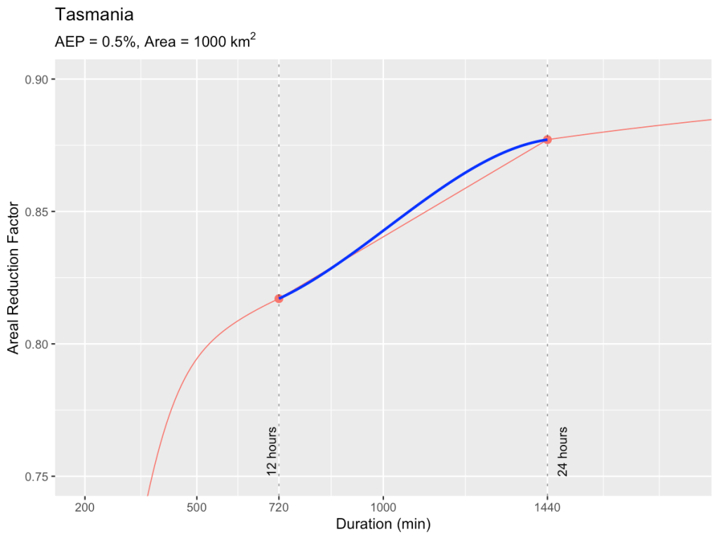
RORB dates from the 1970s and was developed to provide design flood hydrographs usually at a single location at the lower end of a catchment. An example of catchment delineation for a RORB model is show in Figure 1 (left), where a small number of sub-catchments define the set up that can be used to generate a flood hydrograph at node ‘b’. The RORB manual states that between 5 and 20 sub-catchments are sufficient to allow for areal variation of rainfall, losses and the effects of varying flow distance to the catchment outlet. The estimation of RORB parameters for this type of model is reasonably straightforward and is based on the catchment area contributing to ‘b’.

• The design rainfall can be determined by averaging IFD values from the grid of points that covers the catchment.
• Regional relationships can be used to estimate the routing parameter k_c as a function of the catchment area or the dav of the model to ‘b’.
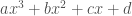
• Areal Reduction Factors (ARFs) are based on catchment area upstream of ‘b’ for a range of durations
• A spatial rainfall pattern can be derived for the catchment based on the grid of IFD values, for AEPs of interest and the corresponding critical durations.

Figure 1: traditional (left), regional (right)

Use of RORB for regional studies

Applying RORB for regional modelling creates several challenges.

More sub-catchments are required

Shifting to a regional focus increases the number of sub-catchments to be modelled. As shown in Figure 1 (right), a RORB model may be required to generate an inflow hydrograph at ‘a’ for a hydraulic model of a flood prone area (inside the green dashed line). The requirement for a minimum of 5 sub-catchments upstream of ‘a’ means that many small sub-catchments must be defined.

Instead of 5 to 20 sub-catchments being required for the whole model, we need at least 5 sub-catchments for every location where a realistic hydrograph is required. The requirement that sub-catchments must be approximately the same size and shape also contributes to the increase in their number.

This means that the total number of sub-catchments in a regional model can become very large. A key issue is that there is interaction between the number of sub-catchments, RORB parameters (such as k_c and losses) and model outputs. I discussed this in an earlier post.

Routing parameters may vary throughout the model

The catchment area of ‘a’ is small so the appropriate k_c value will be smaller than for downstream points such as ‘b’. If model outputs at both ‘a’ and ‘b’, or any other location are required, then different k_c values will be necessary for each location. This can be achieved in RORB by using interstation areas, or by developing separate models for these locations.

A range of Areal Reduction Factors must be considered

There is a similar issue with Areal Reduction Factors. If hydrographs are required at a number of different locations, then the ARFs will depend on the local catchment area of each of these locations. It is not appropriate to choose a single ARF for the whole model.

The specification of design storms will need to vary throughout the model

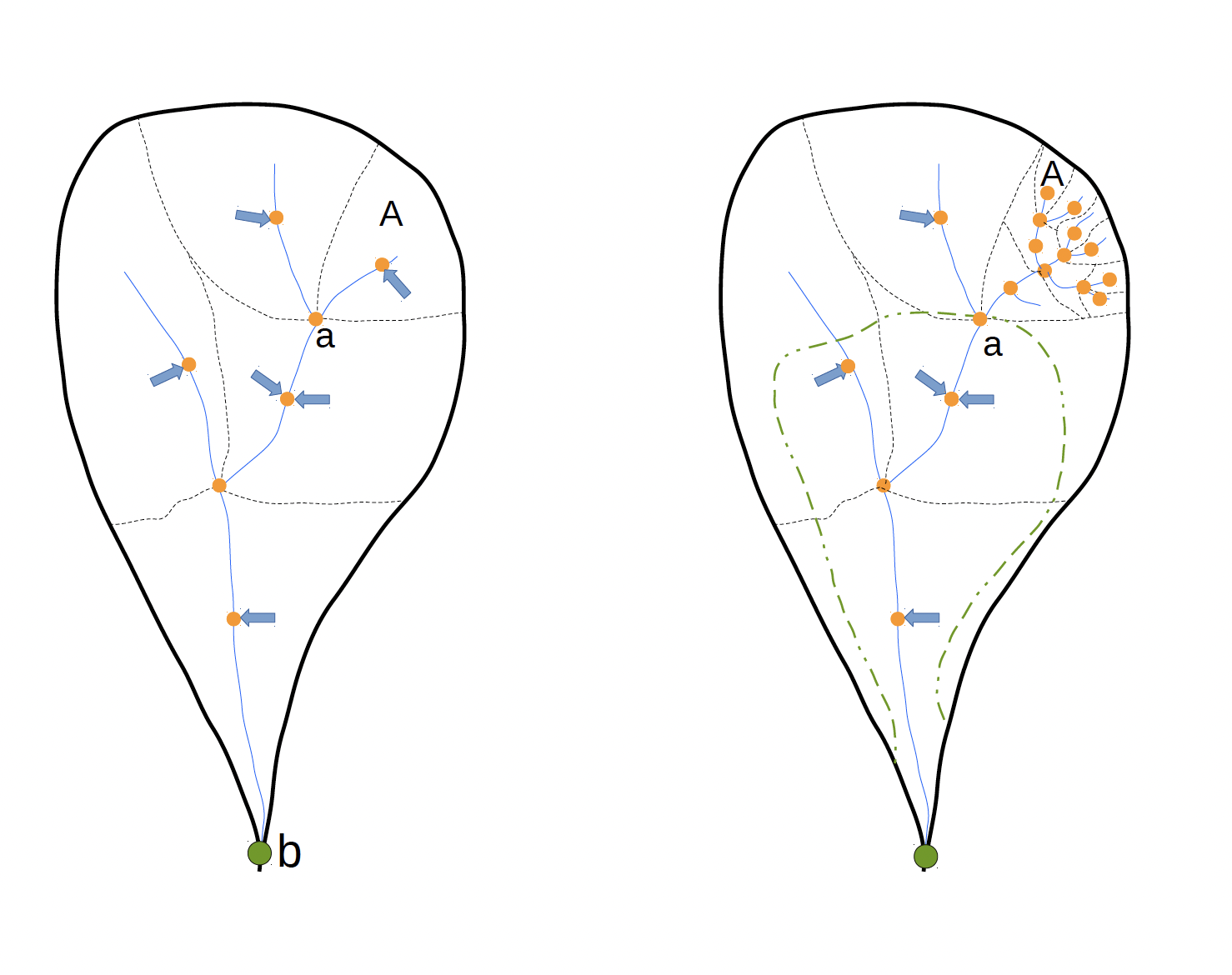
The storm that leads to a design flood (e.g. the 1% AEP flood) will depend on catchment size. Flood runoff from larger catchments is likely to be driven by longer duration, higher volume storms compared to floods from smaller catchments. Therefore, different design storms must be used for different locations.

To emphasise the issue, consider points ‘a’ and ‘b’ in Figure 1 (right). If they are a long way apart and with substantially different catchment areas, it is highly unlikely that a single design storm could define the 1% AEP flood at each location. Conversely, if ‘a’ and ‘b’ are close together and with similar catchment areas then the assumption that a single design storm could be used to characterise a 1% AEP flood at each location is reasonable.

A related issue is defining floods for locations with multiple tributaries. The occurrence of 1% floods in each of the tributary catchment simultaneously is likely to be much rarer than a 1% AEP event. Therefore is not appropriate to model 1% AEP floods in several tributaries and assume that this represents the 1% flood at the location where these tributaries combine.

These issues suggest that one approach to the challenge of modelling appropriate design flood hydrographs would be to divide the area of interest into smaller regions and develop hydrographs for each region based on appropriate design rainfalls depths, ARFs, spatial and temporal rainfall patterns, and routing parameters. These hydrographs would be used as inputs to a hydraulic model of the smaller region. The results from all the regions would need to be stitched together to define flood conditions over the whole area.

In summary, the key messages are:

1. Modelling a design flood hydrograph for a particular location requires appropriate model setup and routing parameters for that location.
2. Similarly, a design storm appropriate for a location must be based on the rainfall depth, spatial pattern, areal reduction factor and losses for the catchment that drains to that location.
3. Quantification of flood risk over a large area is likely to require specific model runs for locations within that area and then the stitching together of the results from these model runs to provide the overall results.

Case study: Effect of a rogue temporal pattern on hydrologic model outputs

I’ve written before about issues with a small number of areal temporal patterns available from the data hub, where there appear to be gross errors.  An example is areal pattern 5644,  Murray-Darling Basin, 36 hour, 500 km² area, 18 x 2 hour increments (Figure 1).

Figure 1: Areal temporal pattern 5644. Murray-Darling Basin, 500 km², 36 hour

Most rainfall (63.6 %), occurs in the 6^th increment (between 10 and 12 hours) and 33.9 % occurs in the final increment (between 34 and 36 hours).  There is 24 hours between the two large rainfalls which suggests an error in the underlying data were a daily rainfall total has been mistaken for a rainfall over a much shorter duration.

So what effect does this have on modelled flood hydrographs?   It turns out this is highly dependent on the continuing loss. 

A ensemble run of RORB model of the Delatite River at Tonga Bridge (1% AEP, 36 hour duration) is shown in Figure 2.  The losses were taken from the data hub: initial loss = 27 mm, continuing loss = 4.3 mm/h.  TPat 8, which has ID 5644, peaks at about 220 cumec, which is 130 cumec more than the next largest hydrograph.

Figure 2: 36 hour ensemble run. Delatite River at Tonga Bridge, IL = 27 mm, CL = 4.3 mm/h

If the CL is reduced to 2 mm/h, TPat 8 no longer dominates (Figure 3). Increasing CL to 7 mm/h means that TPat 8 completely dominates (Figure 3).

Figure 3: 36 hour ensemble run. Delatite River at Tonga Bridge, IL = 27, CL = 2 mm/h

Figure 4: 36 hour ensemble run, Delatite River at Tonga Bridge, IL = 27, CL = 7 mm/h

Embedded burst filtering was turned on for these runs, but the effect of filtering on pattern 5644 was limited (Figure 5). The largest rainfall percentages have been reduced and spread out but two increments still dominate the pattern and the hydrologic response, at least when continuing loss is low.

Figure 5: The effect of embedded burst filtering on pattern 5644

The upshots are:

1. Undertaking an ensemble run with high continuing loss may highlight temporal patterns that require further checking.
2. Turning on embedded burst filtering does not solve the issues associated with temporal patterns that contain gross errors.
3. Hydrologic modellers should considering removing erroneous patterns before undertaken model runs. There is a list of 19 patterns that appear to contain errors here.

New Stream Gauges in the Darling Catchment

An article on 17 Jan 2022 on the ABC mentioned that 20 stream gauges would be installed in response to flooding from the Darling River.

https://www.abc.net.au/news/2023-01-17/nsw-government-installing-water-gauges-menindee-flooding/101860120

I was interested in the cost. There are quotes in the article:

“A typical gauge might cost in the vicinity of $40,000 to $60,000 to install”. “For a river flow site, it will cost on average $15,000 a year to operate”.

This seems a reasonably small amount of money compared to the cost of flood damage. If information from the new gauges could result in a reduction of damage by even a relatively small amount, their installation would be a good investment.

Murray River at Picnic Point on 12 Feb 2023

Improved loss estimation for Victoria

There is now a “Jurisdictional Specifics” page for Victorian on the ARR data hub which is based on a project undertaken by HARC which I was involved in. Our work looked at whether adopting losses from the ARR Data Hub would result in “good” flood estimates from hydrologic modelling. We defined good estimates as when the design flood peaks from modelling are close to the equivalent peaks from flood frequency analysis of gauged data.

In short, the Data Hub losses tend to be too large, which means modelled flood estimates are biassed low. We recommend this is addressed by increasing the preburst rainfall – using the 75th percentile value rather than the median. A caveat is that his recommendation only applies for continuing loss region 3 (see the figure below). There wasn’t enough information to make recommendations for the other loss regions.

Loss regions for Victoria

There is more information available from:

• The Victorian page on the Data Hub
• Our conference paper
• The project report

Of course, the Data Hub isn’t the only source of loss estimates. A key outcome of the project was to develop an ordered list of approaches for estimating losses. Using losses from the Data Hub should only be contemplated when there is no better alternative.

Preferred approaches to loss estimates are, in order:

1. Reconciliation with at-site flood frequency quantiles: initial and continuing losses are varied within their expected range to achieve a reasonable level of agreement between estimates derived from rainfall-based modelling and flood frequency analysis.
2. Reconciliation using within-catchment transposed flood quantiles: streamflow observations are commonly available at gauging stations upstream or downstream of the site of interest, and flood quantiles derived from these sites can be transposed to the site of interest and used for reconciliation as described in approach 1.
3. Event-based calibration: continuing losses obtained from calibration of historical events provide some indication of typical design values, noting that past historical events are biased towards wet catchment conditions; initial losses from historical events are highly variable and information from a small sample of events are of low utility (and therefore some form of reconciliation with other sources of information is recommended).
4. Reconciliation using nearby catchment transposed flood quantiles: regional flood quantiles derived using RFFE and other procedures (Section 3, Book 3, ARR2019) can be used for reconciliation as described in approach 1.
5. Transposition of losses: initial and continuing loss estimates validated on nearby catchments which are considered to be hydrologically similar.
6. Regional losses (ARR Data Hub): unmodified initial and continuing loss estimates obtained from the Data Hub losses can be adopted in data poor areas, noting that in loss region 3 these should be combined with 75^th percentilepre-burst values.

A similar list has also been developed for NSW which, unfortunately, differs from the this one developed for Victoria. The top recommendation from the NSW list is to use calibration losses from the study catchment. Calibration losses are the initial and continue loss that is required to make the output of a hydrologic model match a historical flood peak when historical rainfall is used as the input. This is number 3 on the Victorian list.

Usually, we calibrate to large floods. On average, large floods are likely to have small losses – that is one of the factors that caused the large flood. Therefore, calibration losses may not provide a representative sample of the loss from a catchment; they may be biassed low. Using losses that are biassed low means modelled flood estimates may be too high. Where possible, it would be checking losses through reconciliation with flood frequency analysis of gauged data, using tools such as the RFFE and comparing losses on nearby catchments (Items 2, 4 and 5 on the Victorian list).

A review of temporal patterns from Australian Rainfall and Runoff

Paper presented to the Hydrology and Water Resources Symposium 2021

Abstract

The recommendation in Australian Rainfall and Runoff (ARR) is that an ensemble of 10 rainfall temporal patterns is used for modelling. Patterns depend on region, catchment area and duration and are provided on the ARR Data Hub.  Most available patterns are consistent and appropriate but there are a few which are physically unrealistic and appear to be erroneous.  A method was developed to identify problem patterns and all available areal and point patterns across Australia were checked.  

Nineteen problem areal temporal patterns were identified in 3 regions.  Areal patterns listed on the Data Hub for one region are sometimes borrowed from neighbouring regions and it was found that all the problem patterns originated in the Murray Basin in a small area near Jerangle, 100 km south of Canberra.  The problem seems to be that rainfall accumulated over 24 hours has been allocated to a shorter time step in the pluviograph record.  

This problem means that these patterns are not likely to be suitable for modelling and may lead to unrealistically large flows from long-duration events.  A work around is to exclude these patterns and if necessary, replace them, or use ensembles with fewer than 10 patterns.

Analysis also identified the least uniform point and areal patterns.  These are not necessarily in error but do have the potential to contain “embedded bursts” which occur when a period of rainfall within a temporal pattern has an annual exceedance probability rarer than the burst as a whole.  Embedded bursts can cause issues with modelling and modellers need to consider if they should be removed or smoothed.

Pattern 7 is an example of a ‘problem’ pattern

Region	Duration	Area	Event ID
Central Slopes	48	500	3950
	48	1000	3951
	72	200	4029
	72	500	4043
	72	1000	4049
	96	200	4116
	96	200	4119
	120	200	4207
Murray Basin	36	500	5644
	48	500	5731
	48	500	5732
	72	200	5810
	72	500	5822
	72	1000	5829
	96	200	5901
	96	200	5898
	120	200	5989
Southern Slopes (mainland)	96	200	6797
	120	200	6884

Table 1. List of the 19 problem patterns

Paper

Presentation

Citation:

Ladson, A. R. (2021) Review of temporal patterns from Australian Rainfall and Runoff 2019. 39th Hydrology and Water Resources Symposium. Engineers, Australia.

Can flood control works change a state boundary?

In 1961, Minnesota agreed to ceed land to North Dakota because of a change in course of the Red River of the North as a result of flood control works. Two parcels of land had become detached from Minnesota and attached to North Dakota because of a project undertaken by the US Army Corps of Engineers which cutoff bends of the river.

The State legislatures agreed that State boundaries should be redraw and sought and were granted approval from the US House and Senate. The Minnesota-North Dakota Boundary Line Compact was approved by the US House and Senate on August 25, 1961 as Public Law 87-162. Details are available here.

Both areas are near Fargo North Dakota. The screenshots show the areas and a description of the land is provided in the captions. The maps are sourced from https://www.randymajors.org/township-range-on-google-maps.

NE 1/4 of Section 29, Township 140 North, Range 48 West of the 5th Principal Meridian, Clay County Minnesota (9.78 Acres)

NE 1/4 Section 7, Township 139 North, Range 48 West of the 5th Principal Meridian (12.76 Acres)

Errors in variables regression

The usual assumption in regression is that that all the error is in the y values; the dependent variable; the x values (the independent variable) are known without error.

For a recent project, I had to undertake some analysis where this assumption wasn’t reasonable. There were errors in both variables. In this case, we were looking at the relationship between turbidity and clarity. Turbidity was measured by a meter; clarity was measured as the minimum depth of water that just obscured a target.

As example of the issues, let’s consider a simple case; 10 made up values.

Figure 1: 10 values with random errors around a 1:1 line

For ordinary least squares regression, we calculate a line that minimises the sum of the squared distances between all the points and the line. Only the y distances are considered.

Figure 2: Ordinary least squares finds a line that minimises the sum of the squared distances in the y direction

Next consider the case where the y values are known perfectly all all the error is in the x values. This will give a different regression line.

Figure 3: A different line is obtained if the squared distances are minimised considering only the x-values

We can also consider errors in both x and y values.  Different approaches to this problem are referred to as Errors-in-variables regression, Deming regression or total least squares.  Figure 4 shows the special case of orthogonal regression where the line is calculated by minimising the squared perpendicular distances. This occurs were the variance of the x and y values are equal.  Deming regression can also handle cases where the ratio of the variances is not equal to 1.

The three lines are compared in Figure 5.

Figure 4: Orthogonal regression minimises the sum of the squared perpendicular distances

Figure 5: Comparing the three lines

R code to produce the figures is available as a gist. There is also an example of orthogonal regression in excel available at this link.

On prebust depths and ratios

Preburst rainfall is the rain that falls before a ‘burst’.  Burst rainfall is what you get from IFD information on the Bureau of Meteorology website.  In hydrologic modelling, it is often important to add preburst to burst rainfall to create a ‘design’ storm.

You can look up preburst rainfall on the ARR data hub.   An example is shown below which is for the data hub default location in central Sydney (Longitude = 151.206E, Latitude = -33.87N). These are median preburst values. Data is also available for the 10th, 25th, 75th, and 90th percentiles.

Each cell provides the prebust depth in mm and the preburst ratio (in brackets) for a specified burst AEP and duration.  For example, the top-left cell represents the 50% AEP, 60 min, preburst depth which is 12.0 mm and ratio which is 0.372.  

The ratio is the preburst depth/burst depth.

It’s possible to look up the burst depth, for a given AEP and duration, at the in the IFD website.  

For this location, the 50% AEP, 60 min burst depth is 32.3 mm.  Mutliplying the burst depth by the preburst ratio gives

32.3 x 0.372 = 12.02 mm which is the same as the preburst depth given in the table. 

Sometimes the numbers don’t quite work.  For example the 2160 min (36 hour) burst depth is 357 mm.  With a burst ratio of 0.032, the preburst depth works out to 11.4 mm, compared to 11.6 mm in the table.  A small difference possibly cause by a rounding error or a slightly different IFD values.  The preburst work was based on the interim 2013 IFD data which has since been superseded by the 2016 release.  

Sampling distribution of the 1% flood

A sampling distribution is the probability distribution of a statistic calculated from a sample. In this case, the statistic I’m interested in is the number of floods that may occur in a sample of a certain number of years.

In engineering hydrology, and land use planning, we are often interested in the 1% (1 in 100) AEP flood. If the period of interest is 100 years, say the design life of a house, how many 1% floods should I expect?

We can calculate this using the binomial probability distribution. The general formula is:

Where, n is the number of years (the sample size), p is the probability of a ‘success’ (a flood in this case), r is the number of successes.

So the probability of one 1% flood occuring in 100-years is:

To determine the sampling distribution we need to calculate the probability of getting 0 floods, 1 flood, 2 floods etc. This is shown in Figure 1. The average, or expected number of 1% floods in 100-years is 1, but it’s likely the actual number will be between zero and 4. The probability of getting 5 or more is low, 0.34%

Figure 1: Probability of different number of 1% AEP floods occurring in 100-years

What if our estimate of the 1% flood is not accurate?

Usually the magnitude of the 1% flood is estimated using flood frequency analysis applied to a reasonably short gauge record. Figure 2 shows a flood frequency analysis of 46 years of flood data for the Tyers River at Browns (see this post for details). The best estimate of the 1% AEP discharge is 245 cumec. However, it is quite plausible that this discharge has a true probability of exceedance of 2% rather than 1%.

Figure 2: Flood frequency estimates for the Tyers River at Browns

Consider the scenario where 245 cumec is used for the design flood, and land use planning is based on water levels for this event, however the true exceedance probability is 2% rather than 1%.

The distribution of 2% AEP floods in 100-years is shown in Figure 3. The probability of getting at least 1 flood has increased from 0.63 to 0.87. The probably of getting 5 or more floods has increased by a factor of 15 and is now, 5%. Overall, the risk of flooding has doubled, but the probability of a possibly catastrophic outcome, multiple episodes of flooding, has increased substantially.

Going the other way, if our design flood has a lower AEP value, say 0.5% then the probability of at least one flood drops to 0.39.

Figure 3: Sampling distribution of 2% AEP floods in 100 years

This adds support to taking overall risk into account when selecting design flood levels, rather than just adopting a 1% value and ignoring uncertainty. A risk-based design approach is recommended in Australian Rainfall and Runoff (Book 1, Chapter 5).

This gist has the code to create the figures.

Smooth interpolation of ARF curves

As discussed in the previous post, the areal reduction factors, developed for Australia must be interpolated for durations between 12 and 24 hours. The long-duration equations apply for 24 hours or more. The short duration equations apply for 12 hours or less. In between, the recommendation is to interpolate, linearly (Figure 1) (Podger et al., 2015). This post looks at an alternative to linear interpolation.

Figure 1: Areal reduction factor as a function of duration. ARFs are linearly interpolated between 12 and 24 hours

One approach would be to interpolate in such a way that that there is a smooth curve between the short and long duration values. This can be achieved by matching the slopes, as well as the values, at the end points.

That means there are 4 conditions that must be satisfied. The curve must pass through the two end points and match the slopes (derivatives) at the two end points. This can be achieved with a cubic polynomial.

We have the equations for short and long duration ARFs, and with some help from an on-line differentiator, we can find the derivatives. Its also possible to numerically differentiate the ARF equations.

As in the earlier posts, D is duration (min), P is AEP, A is area in km².

Short duration:

Derivative with respect to duration:

For the long duration equation, the constants, a, b, c, d, e, f, g, h, i, depend on region. See this post for a map of the Australian regions, and the values of the constants.

Long duration:

Derivative with respect to duration:

For the example shown in Figure 1, we have:

AEP = 0.005, Area = 1000 km² Region = ‘Tasmania’.

For a duration of 24 hours (1440 min), long duration ARF = 0.8771, slope = 2.019e-05

For a duration of 12 hours (720 min), short duration ARF = 0.8171, slope = 6.554e-05

A cubic polynomial can be expressed as:

So we need to solve for the four unknowns, using the 4 conditions. In this case the x value is duration.

We can set this up as a matrix equation

Where, x₁ is 720 and x₂ = 1440, f(x₁) = ARF at 720 min, f(x₂) = ARF at 1440 min. f'(x₁) = derivative of the short duration ARF equation at 720 min f'(x₂) is derivative of the long duration ARF equation at 1440 min.

We can then solve for a, b, c and d and draw in the cubic polynomial (Figure 2). The polynomial interpolation doesn’t make a lot of difference but does mean a ‘kink’ in ARF values is avoided.

Figure 2: Polynomial interpolation between 12 hours (720 min) and 24 hours (1440 min)

Code is available as a gist

References

Podger, S., Green, J., Stensmyr, P. and Babister, M. (2015).  Combining long and short duration areal reduction factors. Hydrology Water Resources Symposium (link to paper at Informit).