Tag Archives: 1% flood

1% flood: binomial distribution, conditional probabilities

I previously wrote about considering the occurrence of 1% floods as a binomial distribution, this post extends that analysis to look at conditional probabilities.  Some of the results are counter intuitive, at least to me, in that the risk of multiple 1% floods is larger than I would have guessed.

The probability of a 1% (1 in 100) annual exceedance probability (AEP) flood occurring in any year is 1%.  This can be treated as the probability of a “success”  in the binomial distribution, with the number of trials being the number of years. So the probability of having exactly one 1% flood in 100 years is

{100\choose 1}0.01^{1}\left( 1-0.01\right) ^{99} = 0.37

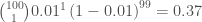
In R this can be calculated as dbinom(x = 1, size = 100, prob = 0.01) or in excel =BINOM.DIST(1,100, 0.01, FALSE).

The cumulative distribution function of the binomial distribution is also useful for flood calculations.

What is the probability of 2 or more 1% floods in 100 years:

R: pbinom(q = 1, size = 100, prob = 0.01, lower.tail = FALSE) = 0.264

Excel: =1 - BINOM.DIST(1,100, 0.01, TRUE) = 0.264

We can check this by calculating the probability of zero or one flood in 100 years and subtracting that value from 1.

1 - (dbinom(x = 1, size = 100, prob = 0.01) + dbinom(x = 0, size = 100, prob = 0.01)) = 0.264

We can also do conditional probability calculations which could be useful for risk assessment scenarios.

What is the probability that exactly two 1% floods occur in 100 years given that at least one occurs?

\Pr{(X = 2\mid X \ge 1)} =
dbinom(x = 2, size = 100, prob = 0.01)/pbinom(q = 0, size = 100, prob = 0.01, lower.tail = FALSE) = 0.291

What is the probability that at least two 1% floods occur in 100 years given that at least one occurs?
\Pr{(X \ge 2\mid X \ge 1)} =
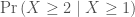
pbinom(q = 1, size = 100, prob = 0.01, lower.tail = FALSE)/pbinom(q = 0, size = 100, prob = 0.01, lower.tail = FALSE) = 0.416

We can also check this by simulation.  This code generates the number of 1% floods in each of 100,000 100-year sequences.  We can then count the number of interest.

set.seed(1969) # use a random number seed so the analysis can be repeated if necessary
floods = rbinom(100000,100, 0.01) # generate the number of 1% floods in each of 100,000, 100-year sequences

floods_subset = floods[floods >= 1] # Subset of sequences that have 1 or more floods
# Number of times there are two or more floods in the subset of 1 or more floods

sum(floods_subset >= 2) / length(floods_subset)
# 0.4167966

# or
sum(floods >= 2)/sum(floods >= 1)

#[1] 0.4167966

A slightly tricker situation is a question like: What is the probability of three or fewer floods in 100-years given there is more than one.

\Pr{(X \le 3\mid X > 1)} = \Pr(X \le 3 \cap X > 1 )/\Pr( X > 1) 

floods_subset = floods[floods > 1] # Subset of sequences that have more than one flood

# Number of times there are three or fewer floods in the subset of more than one flood

sum(floods_subset ≤ 3) / length(floods_subset)
#[1] 0.9310957

# Or, for the exact value

# (Probability that X = 3 + Probability that X = 2)/(Probability that X > 1)
(dbinom(x = 3, size = 100, prob = 0.01) + dbinom(x = 2, size = 100, prob = 0.01))/ pbinom(q = 1, size = 100, prob = 0.01, lower.tail = FALSE)
#[1] 0.9304641


The probability of experiencing at least one 1% flood in 100-years is 1 - (1-0.01)^{100} = 0.634.  How many years would we need to wait to have a 99% chance of experiencing a 1% flood?

0.99 = 1-(1-0.1)^n

n=\frac{log(0.01)}{log(0.99)} = 458.2.  The next largest integer is 459.

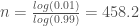
We can also solve this numerically.  In R the formula is 0.99 = pbinom(q=0, size = n, prob = 0.01), solve for n. Using the uniroot function gives n = 459 years (see below).

So all these areas subject to a 1% flood risk will flood eventually, but it may take a while.

f = function(n) {
  n = as.integer(n) #n must be an integer
0.99 - pbinom(q = 0, size = n, prob = 0.01, lower.tail = FALSE) 
}

# $root
# [1] 458.4999

uniroot(f, lower = 100, upper = 1000)

pbinom(q = 0, size = 459, prob = 0.01, lower.tail = FALSE) 
# [1] 0.990079

How many years before there is a >99% chance of experiencing more than one flood? This is one minus (the probability of zero floods + the probability of one flood).

Let the number of years equal n.

1-((1-0.01)^n + n(0.01)(1-0.01)^{n-1}) = 0.99. Solving for n gives 662 years

Calculated Risks

I’ve been reading Calculated risks, a book by Gerd Gigerenzer.  There is lots to make you think.

Here’s an example:

Your DNA matches a trace found on a victim of a crime.  The court calls an expert wetness who gives this testimony:

“the probability that this match has occurred by chance is 1 in 100,000.”

A chance match sounds very unlikely.  So does that mean you will be found guilty?  As Gigerenzer points out, the expert could have phrased the same information as:

“Out of every 100,000 people, one will show a match.”

Now we can see that, in a city like Melbourne, with a population of about 4 million people, about 40 people will show a match.  The point is, that the probability that you committed the crime is not the same as the probability of a match.  The probability that you committed the crime, given the DNA match, is only 1 in 40 if there is no other evidence and the potential perpetrators include anyone living in Melbourne.

Much of the book is about finding clearer ways of talking about, and thinking about, probability and risk.  An example:

The probability that a woman of age 40 has breast cancer is about 1 percent.  If she has breast cancer, the probability that she will test positive on a screening mammogram is about 90 percent.  If she does not have breast cancer, the probability that she will nevertheless test positive is 9 percent.  What are the chances that a woman who tests positive actually has breast cancer?

This is the way Gigerenzer presents the solution, using what he calls, natural frequencies.  Consider 10,000 women, 1% have cancer so that is 100 women.  Of these, 90% will return positive tests (i.e. 90 women with cancer will test positive).  Of the 9900 without cancer 9% will return positive test or 891 women. So there are 891 + 90 = 981 women with positive tests of which 90 have cancer.  So the chance that a woman with a positive test has cancer is 90/981, about 1 in 10.

Cancer.odg 2015-11-22 21-23-33

Different ways of getting a positive test result

We can grind through a problem like this with Bayes theorem but the natural frequency approach makes it easier to understand the problem intuitively.

Bayes

Would the natural frquency idea help with the communication of hydrologic risks?  The latest guidance from Engineers Australia is that we should refer to the 1% annual exceedance probability (AEP) flood rather than the 100-year average recurrence interval (ARI) flood.  This moves away from expressing probabilities as natural frequencies but the rationale is that the ARI terminology is also confusing.  Many people think that only one “100 year flood” can occur every 100 years (see this forum about communicating flood risk in Christchurch, New Zealand)

When discussing flood risk, we could say something like: “Think of your house and 99 other houses, spread all over Australia, that have the same risk of flooding.  On average, one of these houses will flood every year”.

The risk is also the same as rolling a 100-sided die once a year.  If your number comes up, you get flooded.  On average your number will come up every 100 throws but it could come up any throw or several times in a row.

100-sided die

100-sided die (source)

Gigerenzer also talks about absolute risk reduction and relative risk reduction.

If a house is prone to flooding in a 1 in 10 year ARI event (a 10% AEP event) and we build a levee so it is now protected up to the 1 in 100 year ARI event (a 1% AEP event), then the absolute risk reduction is 0.1 – 0.01 = 10% – 1% = 9%.

The relative risk reduction is absolute risk reduction divided by the risk prior to treatment i.e. 0.09/0.1 = 90%.  So if you were to seeking to attract funds for a levee scheme, what sounds better: A 9% absolute risk reduction or a 90% relative risk reduction?

100-year flood: Negative Binomial distribution

The negative Binomial distribution relates to independent trials and provides information on the probability of the number failures before  a certain number of successes. Continuing with our flood examples, the negative Binomial distribution can be used to determine the probability of the number of flood free years before a certain number of floods occur.

If Z is the number of flood free years, before r floods, and if a flood has a probability of occurrence of p in any year then:

Z \sim nbinom(r, p)

Example

A retirement village is vulnerable to the 100-year flood. If there are 3 or more floods in the next 20-years the political pressure will be such that the village will be relocated. What is the probability that this will occur?

Flooded retirement home

Flooded retirement village (http://goo.gl/gtIdcz)


We need the probability that Z + 3 \le 20

The probability can be calculated using R as

pnbinom(17, 3, 0.01) = 0.001

So there isn’t much chance this will happen.

We can also calculate the probability using the Binomial distribution as 1 minus the probability of 2 or fewer flood in 20 years.

1 - pbinom(2, 20, 0.01) = 0.001

The expected value (mean) of Z, the number of flood free years before r floods, is:

\frac{r(1-p)}{p}

Example

What is the average number of years before the retirement village will experience 3 floods?

\frac{3(1-0.01)}{0.01} = 297

This is consistent with the average number of years between 1% floods being 100 years. On average we have 99 flood free years for each event, so in 300 years, on average we will have 297 flood free years and 3 flood events.

Further reading

Jones, O, Maillardet, R. and Robinson, A. (2009) Scientific programming and simulation using R. CRC Press

100-year flood: Geometric distribution – Number of years to the next flood

Here we are interested in the probability distribution of the number of years, Y,  that will elapse before the next 100-year flood occurs. The number of independent trials up, but not including, the first success has a Geometric distribution.  Applying this to flooding means that the number of years to wait before a 100-year flood, has a geometric distribution with the probability parameter equal to 0.01:

Y \sim \mathrm{geom}(0.01)

Example

You have a 5-year assignment to a flood-prone mining camp.  What is the probability that you will experience a 100-year flood while you are living in the camp?

We need the probability that we will wait 4 or fewer years before a 100-year flood.

The probability that you will need to wait n years or fewer is:

\displaystyle \sum _{y=0}^{n} p(1-p)^y

In this case, we interested in:

\displaystyle \sum _{y=0}^{4} 0.01(1-0.01)^y = 0.049

That is, there is a 4.9% chance that the camp will experience a 100-year flood while we are living there.

In R

pgeom(4, 0.01) = 0.049

We can also calculate this using the Binomial distribution as 1 minus the probability of zero floods in 5 years.

1 - pbinom(0, 5, 0.01) = 0.049

The probability that you will be ok for 4 years but be flooded in the 5th year.

P(Y = y) = p(1-p)^n

In this case:

0.01(1-0.01)^4 = 0.0096

Which is 0.96%

In R
dgeom(4, 0.01) = 0.0096

The probability of being flooded increases as the length of our assignment increases as shown in the graph below.

Probability of being flooded as a function of the number of years living in the camp

Probability of being flooded as a function of the number of years living in the camp

We can also plot the probability of being safe for a certain number of years and then being flooded in the next year.

Probability of waiting for a certain number of years and then being flooded in the next year

Probability of being safe for a certain number of years and then being flooded in the next year

Notice that the probability of being flooded in the first year (being safe for zero years) is actually the highest.

Steven Pinker has a nice discussion of this effect in his book ‘The better angels of our nature‘ about 17 pages into Chapter 5.  His discussion uses lightning strikes which I’ve rephrased to floods here.

Suppose that floods are random: every year, the chance of a flood is the same, 1%.  Your house was flooded this year.  When is it most likely you will be flooded again? The answer is next year.  That probability, to be sure, is not very high, 1%.  Now think about the chance you will be safe for a year and then experience a flood the year after next.  For that to happen, two things have to take place.  First, flooding will have to occur the year after next, with a probability of 1%.  Second, flooding will not occur next year.  To calculate that probability you have to multiply the chance there will be no flood next year (0.99 or 1 minus 0.01) by the chance there will be a flood the year after (1% or 0.01).   The probability of these two events occurring is 0.0099, a bit lower than the chance of a flood next year.   What is the chance of being safe for 99 years and then getting a flood? The probability is (1 – 0.99)99 x 0.01 = 10-200, a very small number.

So, if you’ve just experienced a 100-year flood, when are you most likely to experience the next one?  After 100-years? Nope.  The probability is highest that it will happen again next year.  The idea that we’ve had a big flood and will now be safe for a while, is a fallacy.

We can use a random variable drawn from a geometric distribution to simulate the number of safe years before the next 100-year flood occurs.

The mean of a Geometric distribution is

\frac{(1-p)}{p}

In this case, p = 0.01 so the mean number of safe years before a 100-year flood is

\frac{(1-0.01)}{0.01} = 99

On average, we will be safe for 99 years. This is consistent with the idea that the 100-year flood will occur on average once every 100-years.  This may be comforting, but the distribution of the number of safe years isn’t nicely bunched around 99.  The median number of safe years can be calculated using the formula:

\left( \frac{-1}{log_2(1-p)} \right) - 1

In this case, with p = 0.01, the median number of years before the next 1% flood is 68 and the mode (most common value) is zero (i.e. the flood will occur next year). The probability mass values for Y \sim \mathrm{geom}(0.01) are shown below.

Geometric probability mass function (p = 0.01).  The probability that a flood will occur in the year after the indicated number of years without a flood

Geometric probability mass function (p = 0.01). The probability that a flood will occur in the year after the indicated number of years without a flood

Simulating the number of years between floods produces the results shown below (100 simulations in a 10 x 10 grid).  The mean and median are near their theoretical values (i.e. the mean is about 99) but the results show that for many simulations there are a small number of years between floods, while in a few cases there are a very large number of years.

Simulation of the number of years untilla 1% flood occurs. One hundred different random values drawn from a Geometric distribution with p = 0.01

Simulation of the number of years until a 1% flood occurs. One hundred different random values drawn from a Geometric distribution with p = 0.01

We see the same pattern if we simulate a large number of years and randomly determine if a 100-year flood will occur in each year.  A 10,000 year simulation is shown below (100 x 100 year grid). Blue squares show the occurrence of 100-year floods.

A 10,000 year simulation.  Blue blue square show the occurrence of 100-year floods

A 10,000 year simulation (100 x 100 year grid). Blue squares show the occurrence of 100-year floods

The mean and median time between floods are close to their theoretical values, but as we’ve seen before, there are many small gaps between floods and a few very long flood-free periods.  Where dots are close together show periods where floods are clustered.

This type of counter intuitive clustering in random data has been noted in many other situations including the bombing of London during WWII  and the patterns produced by glowworms.  See Pinker (2011) and Gould (1991) for further discussion.

Pinker, S. (2012) The better angels of our nature.  London: Penguin Books. pp 245-247

Gould, S. J. (1991) Glow, big glowworm.  bully for brontosaurus.  New York: Norton (as cited by Pinker)

For R code see this gist.

100-year flood: Poisson distribution

In the previous post we considered the occurrence of 100-year floods as a Binomial random variable. We can do similar analysis using the Poisson distribution.  As noted by Jones et al.  “For n large, the Binom(n,p) distribution is approximately Pois(np)”.

In the examples we’ve been looking at, n is reasonably large i.e. 100 (years).   So binom(100, 0.01) is approximately pois(100 x 0.01) = pois(1).

Lets try it:

Consider the probability of 1, 100-year flood in 100 years.

The poisson distribution can be expressed as follows:

P(X = x) = \frac{e^{-\lambda} \lambda^x} {x!}

In this case, x = 1, \lambda = 1

P(X = x) = 0.367894

So, using the Poisson distribution the probability of 1, 100-year flood in 100 years is 0.367894. Using the Binomial distribution it is 100 x 0.01 x (1-0.01)^99 = 0.3697296. i.e. pretty close. The approximation gets better for larger n.

Similar to the Binomial example, we can use a Poisson random variable to simulate flood occurrence – although the Binomial approach will be more accurate.  The figure below shows a simulation of 100, 100-year sequences in a 10 x 10 grid.  You can see that most of the time there is 0 or 1 flood but occasionally there are a lot more.

Simulation of the number of 100-year floods occurring in 100 (10 x 10), 100-year sequences.

Simulation of the number of 100-year floods occurring in 100 (10 x 10), 100-year sequences

R code (also available as a gist)

 
dpois(0,1)  # prob of zero 100-year floods in 100 years
[1] 0.3678794
dpois(1,1)  # prob of one 100-year floods in 100 years
[1] 0.3678794
dpois(2,1)  # prob of two 100-year floods in 100 years
[1] 0.1839397


# simulation

library(ggplot2)
df <- expand.grid(x = 1:10, y = 1:10)
df$z <- rbinom(100, 100, 0.01) # could also use rpois(100,1)


ggplot(data=df, aes(x,y)) + geom_tile(aes(fill=z)) + 
  scale_fill_gradient(low="green", high = "red", name = 'Floods') +
  geom_text(data = df, aes(x, y, label = z)) +
  scale_x_continuous(breaks = NULL) +
  scale_y_continuous(breaks = NULL) +
  xlab('') +
  ylab('') 


set.seed(2000)
rpois(10, 1)
[1] 0 1 0 1 2 1 3 1 2 1
# number of 100-year floods in each of 10 100-year sequences


100-year flood: Binomial distribution

The Binomial distribution applies when there are trials with two outcomes (‘success’ and ‘failure’).  The standard example is coin tossing; a coin can come up heads or tails and the probability of success e.g. a head, is the same in every trial.  The probability of tossing a head with an unbiased coin is 50% but the binomial distribution also applies where the probability of success differs from 50%.  In the case of a 100-year flood, the probability of ‘success’ – having a 100-year flood, is 1% in any year.

The Binomial distribution can be used to calculate the probability of experiencing a certain number of 100-year floods in a specified number of years.  The probability of  experiencing 0, 1, 2, 3, 4 or 5 100-year floods in 100 years is shown in the table and figure below.  Having one flood is the most likely outcome but there is also a good chance of having zero, or 2, or more.  There is a 63.4% change of having at least 1.

Number of floods Probability
0 36.6%
1 37.0%
2 18.5%
3 6.1%
4 1.4%
5 0.3%
At least 1 63.4%
Probability of experiencing 0, 1, 2, 3, 4 or 5 100-year (1%) floods in 100 years

Probability of experiencing 0, 1, 2, 3, 4 or 5 100-year (1%) floods in 100 years

Lets do a sample calculation.  The probability of k successes from n trials, where the probability of success from an individual trial is p, is given by:

{n\choose k}p^{k}\left( 1-p\right) ^{n-k}

So the probability of exactly two, 100-year floods in 100 years is:

{100\choose 2}0.01^{2}\left( 1-0.01\right) ^{98} = 0.185 or 18.5%

The probability of at least one flood is the same as 1 – the probability of zero floods. So the probability of at least one 100-year flood in 100 years is:

1-(1-0.01)^{100} = 0.6339677 \approx 1 - \frac{1}{e}

We can also use a Binomial random variable to simulate the occurrence of floods.  Check the help for ?rbinom.

To simulate the number of 100-year floods in 100 years:

rbinom(1, 100, 0.01)

To do this in 10, 100-year sequences:

rbinom(10, 100, 0.01)

See the code below for an example.

R code (also available as a gist)

dbinom(0,100,0.01) # zero 1% floods in 100 years
dbinom(1,100,0.01)
dbinom(2,100,0.01)
dbinom(3,100,0.01)
dbinom(4,100,0.01)
dbinom(5,100,0.01) # five 1% floods in 100 years

# at least 1 1% flood in 100 years
1 - pbinom(0,100, 0.01) 

# Sample calculation
# Exactly 2 1% floods in 100 year
choose(100,2) * 0.01^2 * (1 - 0.01)^98
#[1] 0.1848648


par(oma = c(1, 2, 0, 0))
barplot(dbinom(0:5,100,0.01),
        ylim = c(0, 0.4),
        las = 1, 
        names.arg = 0:5,
        ylab = 'Probability',
        xlab = 'Number of 100-year floods in 100 years')

set.seed(2000)
rbinom(10, 100, 0.01)
#[1] 0 1 0 1 2 1 3 1 2 1
# number of 100-year floods in each of 10 100-year sequences