I’ve been reviewing some of the background that explains the way RORB works, particularly Appendix A in the RORB manual and the 1974 paper by Mein, Laurenson and McMahon Simple Nonlinear Model for Flood Estimation.
The key mathematical aspects of RORB are the continuity equation and a relationship between storage and discharge.
For any storage, the continuity equation can be written as: “inflow in a time period, minus outflow in that time period equals change in storage”.
Or as used in RORB:

Where 


The relationship between storage and discharge used in RORB is:

This is justified in Appendix A of the RORB manual and in Mein et al. (1974).
Substituting equation (2) into (1):
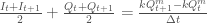
In the general case, we are solving for the outflow 


Equation (3) can be rearranged as follows

I’ve written that equation (4) is equal to zero, but this will only be the case if we have the correct value of
This opens the possibility of a numerical solution; guess a value of
Let’s start with the Newton-Raphson procedure which the method discussed in Mein et al. (1974)
Think of equation (4) as a function of

We guess a value of 


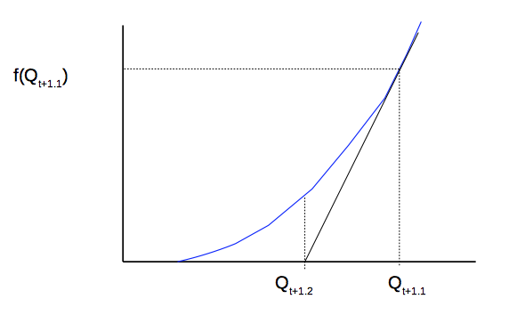
The slope is rise/run so in this case.
Now, rearrange (6) to give an expression for
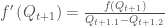
Next we need the derivative of equation (5) with respect to
Using this approach to find

Equation (9) is the same as equation (8) in Mein et al. (1974).
The iterative solution proceeds as follows.
- Select an initial value of
for the first timestep
,
- Guess
(Mein et al. use
- Use equation (9) to calculate
- Set
- Calculate a new
- Repeat steps 3 to 5 until
- Go to the next timestep
- Set
(current timestep) equal to
- Repeat steps 2 to 8 for all time steps

This sounds straightforward but there can be numerical issues. The initial guess needs to be quite close to the answer or the next guess provided by equation (9) could be a negative flow. Putting this back into equation (5) will cause an error because it requires raising a negative number to a fractional power. Another challenge is that the derivative (equation 8) is undefined when 

When reading the RORB manual, section 2.2.5 there is a comment that: “The Regular Falsi convergence algorithm was used”. There is a good description of this root finding approach in Wikipedia. The upshot is that RORB does not use Newton-Raphson as was discussed in Mein et al. 1974.
In R, the uniroot function provides a reliable way of root finding without the numerical issues of the Newton-Raphson procedure. uniroot is based on a C function zeroin as documented here.
A simple routing function, in R, is below.
Routing <- function(Ihydrograph, k, m, T, dt = 1, plotit = TRUE, return.values = FALSE){

# Ihydrograph is a function that describes the inflow hydrograph
# k and m are the routing parameters
# dt is the time step

 I <- rep(0, T+1) # Initialise input vector
 Q <- rep(0, T+1) # Initialise output vector
 S <- rep(0, T+1) # Initialise storage vector


 I[1] <- Ihydrograph(1) # initialise inflow

 # Continuity equation that we seek to set to zero to determine Q at the next time step

 myF <- function(Qip1, Qi, Ii, Iip1, k, m, dt){

 Qip1 + Qi - Iip1 - Ii + (2*k/dt)*(Qip1^m - Qi^m)

 }


 for(i in 1:100){
 I[i+1] <- Ihydrograph(i+1)
 Q[i+1] <- uniroot(myF, interval = c(0,10), Qi = Q[i], Ii = I[i], Iip1 = I[i+1], k, m, dt)$root
 S[i+1] <- k*Q[i+1]^m

 }


 if(plotit){
 plot(I, type = 'l', col = 'blue', las = 1, ylab = 'flow', xlab = 'Time step') # Inflow hydrograph
 lines(Q) # outflow hydrograph
 legend('topright', legend = c('Inflow', 'Outflow'), lty = 1, col = c('blue', 'black'), bty = 'n' )
 }

 if(return.values) return(Q)

}
Let’s test it using a hydrograph as a function (see this blog for details).
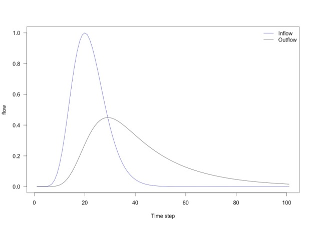
What about the influence of k on routing?
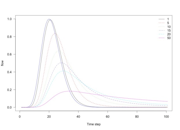
Influence of the k parameter on routing
RORB starts with a rainfall excess hyetograph (the rainfall that is left over after losses have been subtracted) and then routes this through a series of elements to produce flow at the catchment outlet. Here I’ve modelled a single element but that gives an indication of how the program works.
Code for the routing function and to produce these figures (also available as a gist).
Code to produce these figures.
# Specify an inflow hydrograph as a function
# See https://tonyladson.wordpress.com/2015/07/21/hydrograph-as-a-function/

my.Qmin <- 0
my.Qmax <- 1
my.beta <- 10
my.t.peak <- 20

Hydro <- function(tt, t.peak = 3, Qmin = 1, Qmax = 2, beta = 5) {
Qmin + (Qmax - Qmin)*( (tt/t.peak) * (exp(1 - tt/t.peak)))^beta

}
# Initialise the inflow
Ihydrograph <- function(tt){
Hydro(tt, t.peak = my.t.peak, Qmin = my.Qmin, Qmax = my.Qmax, beta = my.beta)
}

# Routing
Routing(Ihydrograph, k = 20, m = 1, T = 100, plotit = TRUE, return.values = FALSE)
# Step function hydrograph (or possibly based on measured inflows)

inflow <- c(0,0, 1,1,1,1,1, rep(0, times = 94))
Ihydrograph <- approxfun(1:101, inflow)
Routing(Ihydrograph, k = 20, m = 1, T = 100, plotit = TRUE, return.values = FALSE)


############################################
# Influence of k

# Wrap Routing as a function of k

Routing_k <- function(k, Ihydrograph, m, T, dt = 1, plotit = TRUE, return.values = FALSE){
Routing(Ihydrograph, k, m, T, dt = 1, plotit = plotit, return.values = return.values )
}
k.seq <- c(1, 5, 10, 15, 20, 50)
x <- lapply(k.seq, FUN = Routing_k, Ihydrograph = Ihydrograph, m = 0.8, T = 100, dt = 1, plotit = FALSE, return.values = TRUE)
x1 <- do.call(cbind, x)

plot(Ihydrograph(1:100), type = 'l', col = 'blue', las = 1, ylab = 'flow', xlab = 'Time step') # Inflow hydrograph
matlines(x1)
legend('topright', legend = k.seq, col = 1:6, lty = 1:5, bty = 'n' )

Pingback: Routing in RORB – II | tonyladson